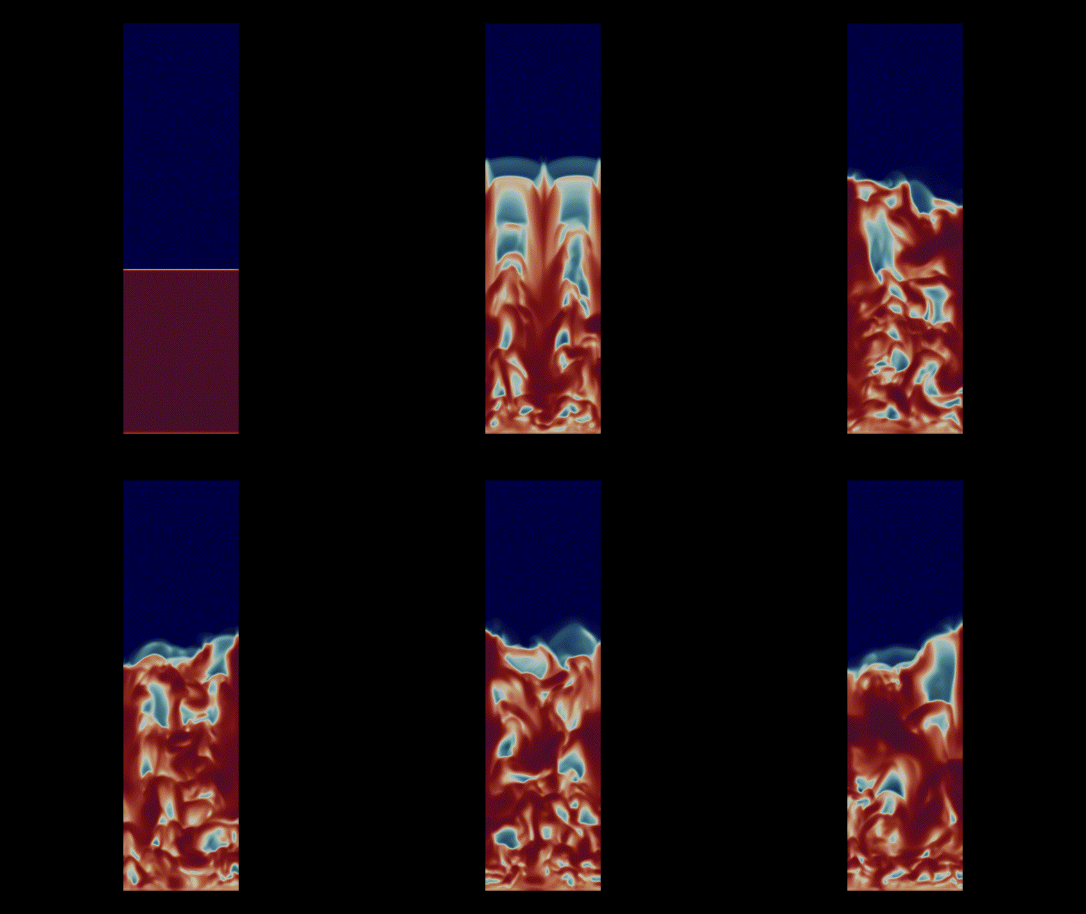
Description: Transient turbulent Euler–Euler simulation of a fluidized bed
Reference Paper: Experimental and computational study of gas-solid fluidized bed hydrodynamics
Model
The model consists of a rectangular domain of width 0.28 m, height 1 m, and depth 0.025 m.
The initial solids height was 0.4 m, with an initial solid fraction ($\alpha_s$) of 0.6 and a maximum solid fraction of 0.63.
Meshing
Meshing was performed using blockMesh.
The resulting mesh had 498,443 points and 448,000 hexahedral cells.
Physics
The model was simulated using the two-phase Euler–Euler model, which assumes continuum mechanics for both the fluid phase—in this case, gas—and the solid phase.
RAS models were used to compute the turbulence in both phases.
The $k-\epsilon$ model was used for closure of the turbulence stress in the gas phase.
For the solid phase, Kinetic Theory of Dense/Granular Flows (KTGF) was used to close the momentum equations.
The table below provides information about the models used for closure of the equations.
| Closure | Model |
|---|---|
| Momentum drag exchange ($K_{gs}$) | GidaspowErgunWenYu |
| Heat transfer | RanzMarshall |
| Granular viscosity | Gidaspow |
| Granular conductivity | Gidaspow |
| Granular pressure | Lun |
| Frictional stress | JohnsonJacksonSchaeffer |
| Radial model | SinclairJackson |
Simulation
The case was simulated using the multiphaseEuler solver in OpenFOAM.
Some important parameters and their values are given in the table below.
| Parameter | Value | Comment |
|---|---|---|
| Particle density, $\rho_s$ | $2500\ \mathrm{kg/m^3}$ | Glass beads |
| Gas density, $\rho_g$ | $1.225\ \mathrm{kg/m^3}$ | Air |
| Mean particle diameter, $d_s$ | $275\ \mu\mathrm{m}$ | Uniform distribution |
| Restitution coefficient, $e_{ss}$ | $0.95$ | Range in literature: 0.9–0.99 |
| Specularity coefficient, $e_{sp}$ | $0.2$ | For the particle wall condition |
| Initial solids packing, $\epsilon_{s0}$ | $0.6$ | Fixed value |
| Maximum solids packing, $\epsilon_{s,\mathrm{max}}$ | $0.63$ | Fixed value |
| Superficial gas velocity, $U$ | $0.38\ \mathrm{m/s}$ | Approximately $0.5$–$6U_{mf}$ |
Boundary Conditions
| Parameter | Internal Field | Inlet | Outlet | Walls |
|---|---|---|---|---|
| U.particles | uniform (0 0 0) |
interstitialInletVelocity uniform (0 0.38 0); alpha.air |
pressureInletOutletVelocity; phi.air |
noSlip |
| U.air | uniform (0 0 0) |
fixedValue uniform (0 0 0) |
fixedValue uniform (0 0 0) |
JohnsonJacksonParticleSlip |
| Pressure ($p_{rgh}$) | uniform 1e5 |
fixedFluxPressure value = 1e5 |
prghPressure; value = 1e5 |
fixedFluxPressure; value = 1e5 |
| alpha.air | Set using setFields |
zeroGradient |
zeroGradient |
zeroGradient |
| alpha.particles | Set using setFields |
zeroGradient |
zeroGradient |
zeroGradient |
| Theta.particles | uniform 0 |
fixedValue; value = 1e-4 |
zeroGradient |
JohnsonJacksonParticleTheta |
| k.air | uniform 1 |
fixedValue; value = 1 |
inletOutlet |
kqRWallFunction |
| epsilon.air | uniform 10 |
fixedValue; value = 10 |
inletOutlet |
epsilonWallFunction |
The transient simulation was run for 5 s with an adaptive time step of $\Delta T = 0.0001$ using the PIMPLE (PISO/SIMPLE) algorithm.
The PISO algorithm was used with three non-orthogonal correctors and two correctors, along with drag correction.
Validation
The results were validated against the reference paper mentioned above.
The important validation parameters were the expansion ratio $\frac{H}{H_0}$ and the pressure drop $\Delta p$.
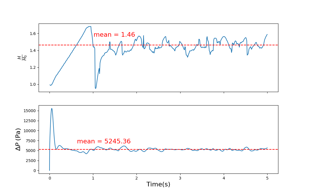
Since the system exhibited oscillatory behavior after approximately 2 s, the time range from 3 s to 5 s was used to compute the mean values.
The mean expansion ratio and pressure drop were calculated over this time range. These values are provided below along with the reference values.
| Parameter | Simulation | Reference |
|---|---|---|
| $\frac{H}{H_0}$ | 1.46 | 1.49 |
| $\Delta p$ (Pa) | 5245 | 5428 |
From the table above, it can be inferred that the simulation was successfully validated and that fluidization was successfully observed.